Education of Disadvantaged Children in OIC:
The Key to Escape from Poverty
246
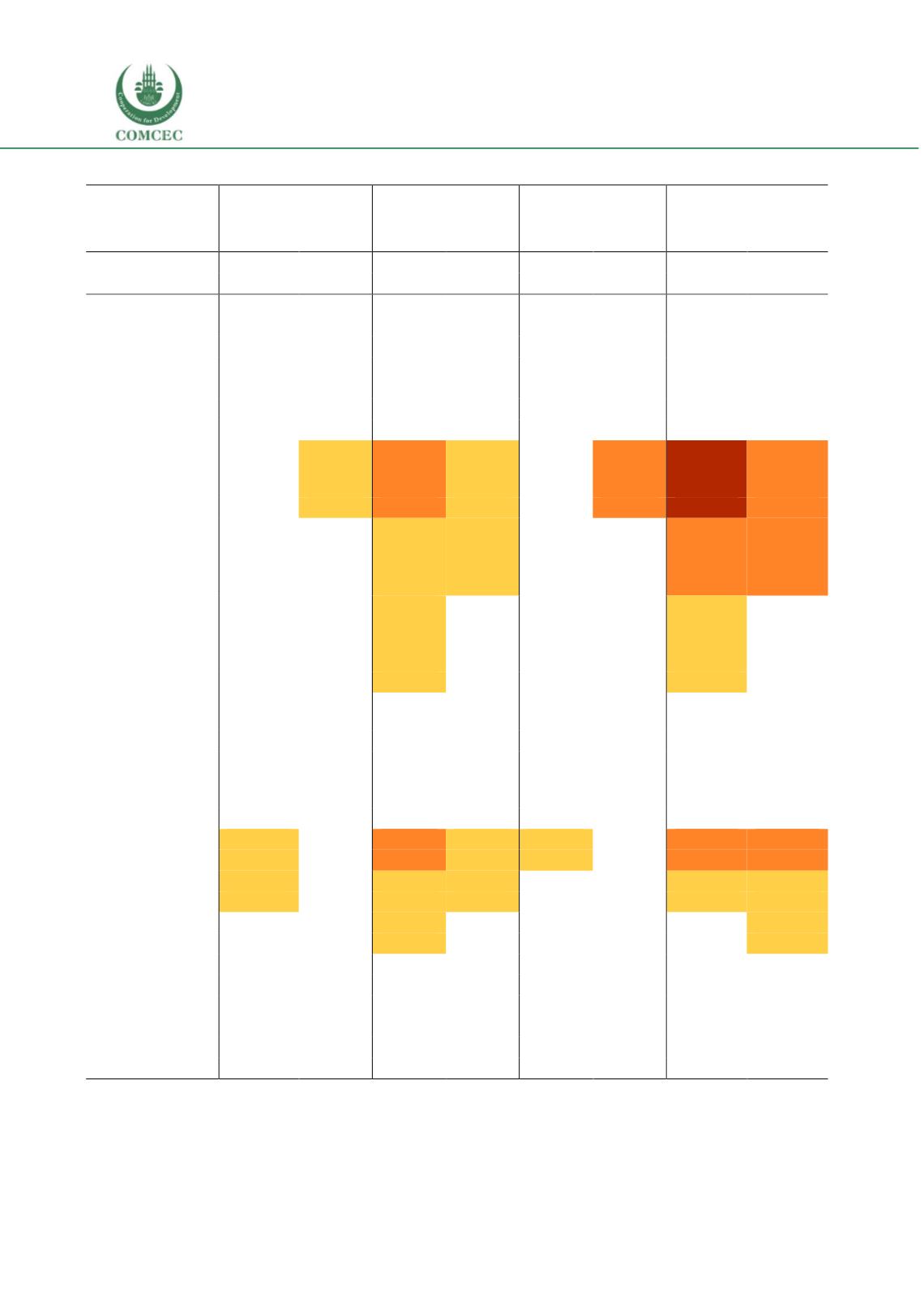
Annex Table 6 Probit regression results (reporting marginal effects)
Attendance 6-11 year
olds
Attendance 12-15
year olds
Finishing 5 years of
education
(12-15 year olds)
Finishing 8 years of
education
(16-18 year olds)
(1) (2) (3) (4) (5) (6) (7) (8)
VARIABLES 1997 2012 1997 2012 1997 2012 1997 2012
location: Rural 0.007 0.003 0.015* 0.025*** 0.008* 0.007** 0.018 0.018***
(0.011) (0.003) (0.008) (0.005) (0.005) (0.003) (0.015) (0.006)
region: North -0.005 0.003 0.024*** 0.006 0.005 0.002 0.006 0.020***
(0.010) (0.004) (0.008) (0.006) (0.005) (0.003) (0.015) (0.006)
region: South -0.027** 0.008*** 0.018* 0.020*** -0.011 -0.000 -0.015 0.022***
(0.013) (0.003) (0.010) (0.005) (0.013) (0.004) (0.027) (0.006)
household head’s
education: No
education
0.007 -0.066*** -0.156*** -0.168*** -0.022* -0.101*** -0.220*** -0.188***
(0.015) (0.023) (0.037) (0.041) (0.013) (0.031) (0.045) (0.049)
household head’s
education: Primary
education
0.003 -0.023** -0.092*** -0.064*** 0.001 -0.026*** -0.118*** -0.111***
(0.010) (0.010) (0.023) (0.017) (0.007) (0.010) (0.029) (0.025)
household head’s
education:
Secondary
education
-0.005 -0.005 -0.052*** -0.014* 0.001 -0.003 -0.095*** -0.026***
(0.010) (0.004) (0.018) (0.007) (0.006) (0.004) (0.026) (0.009)
# of children in
household: 3-4
-0.003 0.005 0.010 0.004 -0.004 0.002 0.018 0.003
(0.013) (0.004) (0.008) (0.005) (0.005) (0.003) (0.013) (0.006)
# of children in
household: 5 or
more
0.022 -0.002 -0.001 -0.010 -0.002 -0.003 -0.005 -0.002
(0.014) (0.004) (0.009) (0.007) (0.005) (0.004) (0.013) (0.008)
wealth: Poorest -0.061*** -0.029** -0.101*** -0.084*** -0.062*** -0.008 -0.115*** -0.111***
(0.017) (0.012) (0.028) (0.021) (0.019) (0.007) (0.034) (0.035)
wealth: Poorer -0.051*** -0.013 -0.054** -0.064*** -0.030** -0.010 -0.058** -0.081**
(0.015) (0.009) (0.022) (0.020) (0.014) (0.008) (0.028) (0.033)
wealth: Middle -0.019 -0.024** -0.052** -0.042** -0.004 -0.002 -0.048* -0.054*
(0.014) (0.012) (0.023) (0.018) (0.009) (0.007) (0.028) (0.031)
wealth: Richer -0.015 -0.004 -0.018 -0.009 -0.001 0.009* 0.025 -0.014
(0.012) (0.008) (0.017) (0.014) (0.009) (0.005) (0.022) (0.023)
gender: Female 0.005 0.002 0.001 0.003 -0.006 0.004 0.016 0.022***
(0.007) (0.002) (0.006) (0.004) (0.004) (0.003) (0.012) (0.005)
Observations 7,251 11,501 4,470 6,966 4,470 6,966 2,849 4,748
Note: Authors’ calculations using DHS 1997 and DHS 2012. Marginal effects are reported, obtained using “dprobit”
command in STATA. Robust standard errors in parentheses. *** p<0.01, ** p<0.05, * p<0.1. Omitted groups are: